BaC SERICS (SEcurity and RIghts In theCyberSpace) – SPOKE 8

(from 10/5/2024 to 30/9/2025)

Project team

University of Parma – Prof. Francesco Zanichelli (PI)

University of Parma – Prof. Luca Veltri (co-PI)

University of Parma – Prof.  Michele Amoretti

University of Parma – Prof. Stefano Caselli

University of Parma – Prof. Giulio Colavolpe

University of Parma – Dott.ssa Eleonora Iotti

University of Parma – Prof. Monica Mordonini

University of Parma –Dott. Gabriele Penzotti

University of Parma – Dott. Alessio Russo

University of Parma – Prof.  Michele Tomaiuolo

Project summary

ASSIST aims to study and propose an enhanced IIoT distributed architecture with new security mechanisms/components addressing some of the challenging issues in the software vulnerabilities of these critical industrial systems.

The main research activities focus on:

1. Detection components:  design of proper security components targeting the detection of possible
   vulnerabilities and attack attempts, also leveraging upon state-of-the-art Machine Learning methods and tools, such as Large Language Models;
2. Architecture for Secure M2M Interactions:  design of proper security components that can be used to enhance the overall security of the systems by guaranteeing both the security of the interactions in terms of entity authentication and authorization, and the protection of the data in terms of data integrity, confidentiality and access control.
3. Implementation and Tests: all ASSIST detection components will be separately implemented and tested. A performance campaign will be carried out and results will be analysed to validate the proposed solutions and to tune possible system parameters.

Workpackages

WP Nr.	Description
WP0 – Management and reporting	Technical and administrative coordination, reporting and dissemination.
WP1 – Detection Components	IIoT vulnerability assessment and anomaly/intrusion detection using Machine Learning and Large Language Model techniques.
WP 2 – Architecture for Secure M2M Interactions	Securing M2M communications, by providing data integrity and confidentiality, and peer entity authentication, authorization, and access control.
WP3 – Implementation and Tests	Implementing and testing the new components and the proposed architecture.

Final Technical Report

Table of contents

1       Scope. 3

2       Scenario. 4

2.1         Reference scenario. 4

2.2         Security framework and main components. 6

2.2.1          Goals and Design Principles. 6

2.2.2          Security components. 7

3       E2E security. 8

3.1         M2M communication protocols. 8

3.2         E2E data protection. 10

3.3         Group key management. 11

3.3.1          Slotted group key management. 12

3.4         MQTT extension for E2E security. 14

3.4.1          MQTT with STATIC Group Key Distribution. 14

3.4.2          MQTT with UPDATE Group Key Distribution. 15

3.4.3          MQTT with SLOTTED Group Key Distribution. 16

3.5         CoAP extension for E2E security. 17

3.6         Implementation. 18

3.6.1          KD Server. 18

3.6.2          Secure MQTT. 18

3.6.3          Secure CoAP. 19

3.6.4          Embedded devices. 19

4       Anomaly detection. 20

4.1         Anomaly detection in IIoT. 20

4.2         Goal and functional description. 20

4.2.1          Functional description. 21

4.3         Implementation. 23

4.3.1          Data Preprocessing and Feature Engineering. 24

4.3.2          Machine Learning Models. 25

4.4         Experimental Results. 25

4.4.1          Cross-Validation on Independent Dataset. 27

5       Source Code Vulnerability Detection. 29

5.1         Context and Goals. 29

5.1.1          Functional description. 29

5.1.2          Component Design. 30

5.2         Implementation. 36

5.2.1          Overview.. 36

5.2.2          Technology Stack and Tooling. 38

5.2.3          Module-wise Implementation Details. 38

5.2.4          Vulnerability Detection Strategies. 43

5.2.5          Deployment Scenarios. 46

5.2.6          Testing the system.. 47

5.2.7          Limitations and Extensions. 47

6       Malware detection. 49

6.1         Context and goals. 49

6.1.1          Objectives. 49

6.1.2          Functional description. 50

6.2         Implementation. 50

6.2.1          Feature Space Exploration. 51

6.2.2          Minimal Change Analysis. 52

7       References. 54

8       Publications. 55

8.1         Submitted articles. 55

1       Scope

The transition to Industry 4.0 is driving the emergence of fully automated and interconnected industrial production environments. In this scenario, industrial cyber-physical systems are deeply integrated with operational, control, and management infrastructures, resulting in highly heterogeneous system architectures. Given the critical nature of both the information handled and the underlying production infrastructure, cybersecurity has become a key concern.

However, securing such complex and interconnected environments poses significant challenges due to several factors:

• Device Heterogeneity: A wide range of devices—such as sensors, actuators, PLCs, and SCADA systems—operate using IoT and industry-specific protocols. Many of these devices are resource-constrained, with limited memory and processing power, and may have inherent vulnerabilities.
• Protocol Diversity: These systems often rely on specialized, and sometimes proprietary, communication protocols that were originally designed for use in isolated or protected networks, lacking robust built-in security.
• Software Lifecycle Complexity: Applications in these environments may not be thoroughly tested, and applying patches or updates can be difficult, leaving systems exposed to known vulnerabilities.

In response to these challenges, the ASSIST project aimed to design and propose an enhanced architecture for the Industrial Internet of Things (IIoT) with integrated security mechanisms. Specifically, the project will focus on developing new components to:

• Secure M2M Interactions: Implement data-oriented authentication, access control and confidentiality for machine-to-machine communication.
• Enable Anomaly and Intrusion Detection: Introduce ML-based automated methods to identify anomalies and potential intrusion attempts.
• Software Security Assessment: automated ML-based methods for identifying possible software vulnerabilities and for malware detection.

2       Scenario

2.1      Reference scenario

Historically, traditional industrial production systems were composed of distinct, highly segmented subsystems. These systems connected local devices and control components—such as sensors, actuators, PLCs, and SCADA—through specialized operational technology (OT), often relying on proprietary protocols and custom-built mechanisms.

Because these OT subsystems typically operated in isolation from industrial IT infrastructure and did not interact with other Internet-connected systems, the risk of external cyberattacks was low. As a result, security was not a primary consideration in the design or selection of communication technologies and OT software development. Instead, priorities were placed on achieving real-time performance (with minimal latency) and ensuring high reliability.

However, with the advent of Industry 4.0, this landscape has shifted dramatically. OT systems are now increasingly integrated with IT networks, and some may even connect to external, cloud-based platforms for continuous monitoring, remote maintenance, and software or firmware updates.

This evolution has given rise to a complex and heterogeneous IP-based network in which traditional OT components are tightly coupled with both local and remote IT systems. In Figure 1 an example of Industry 4.0 interworking scenario is depicted. In such an interconnected environment, relying on strict segmentation and isolation for security is no longer sufficient.

Figure 1 – Industry 4.0 networking scenario.

While securing Internet-connected systems is a well-established area—with widespread use of tools like secure communication protocols, firewalls, intrusion detection systems (IDS), and antivirus software—most of these solutions were originally developed for traditional IT environments.

However, Industry 4.0 introduces a very different context. The nature of connected devices, communication technologies, applications, and operational requirements differ significantly from conventional IT systems. As a result, ensuring security in this new industrial landscape is far more complex, giving rise to new challenges.

Several key factors contribute to the difficulty of securing industrial systems:

• Highly heterogeneous networks that integrate both OT (Operational Technology) and IT components;
• Diverse OT devices (such as sensors, actuators, PLCs, SCADA systems), often built with custom hardware, firmware, and software, each potentially carrying unique vulnerabilities;
• Resource-constrained devices, which may have limited computing power, memory, or network capabilities. These limitations can hinder the implementation of modern security mechanisms. Many devices also lack user interfaces, making configuration changes or updates difficult or even impossible;
• Use of IoT and industrial-specific protocols, including proprietary ones that were originally designed for isolated, trusted environments and not for open, interconnected systems;
• Poorly tested application implementations, often based on proprietary or undocumented software, with complex update and patching processes that increase exposure to threats;
• Multiple attack surfaces and vectors, even in physically isolated environments. Threats can emerge through wireless connections, unsecured physical access ports, the accidental or intentional connection of compromised devices (e.g., laptops or smartphones), or unauthorized physical access.

In this project, we considered an Industrial scenario where different production lines on different sites may be connected to the IT infrastructure and to possibly third parties that provide remote services. Each production facility may house several production lines consisting of diverse machinery, as depicted in Figure 2.

Figure 2 – Considered industrial infrastructure scenario.

The monitoring and control of this machinery is provided by the deployment of OT systems such as PLCs, SCADA, and distributed sensing networks composed of IIoT devices. These systems are interconnected to remote controllers at the line and site levels. Furthermore, these controllers can be linked to corporate headquarters or external cloud infrastructure to enable cross-site monitoring and control. Collectively, these components form a complex IIoT network, which may necessitate interconnection with external entities, like machine manufacturers or third-party maintenance firms.

Regarding communication technologies, current industrial systems utilize either proprietary ad-hoc solutions and/or standard protocols. The adoption of standard protocols offers distinct advantages concerning interoperability, scalability, and long-term maintainability. Among these standards, the publish/subscribe (pub/sub) communication paradigm is particularly promising. In this model, data producers publish information to a central server, which then distributes it to various data consumers.

Within the IIoT domain, MQTT has emerged as the de facto standard for implementing the pub/sub paradigm. It serves dual purposes: collecting data from diverse sources like PLCs and sensors, and dispatching commands from controllers to target devices. Typically, the pub/sub mechanism relies on a central node, termed as broker in MQTT notation, which receives published data and selectively relays it to the appropriate subscribers.

It can generally be assumed that machines from the same manufacturer might share a common communication system centered around a single broker. This configuration can lead to the presence of one or more brokers per production line, potentially resulting in multiple brokers operating within a single site.

To ensure adequate protection and isolation of distinct information flows, the implementation of a robust dynamic authentication and authorization system is necessary. However, this task is complicated by the potentially large number of machine-to-machine (M2M) interactions requiring individual consideration. Furthermore, at a lower network level, these interactions demand explicit configuration on intermediate devices such as NATs and firewalls.

Consequently, the resulting overall framework can become highly complex, exhibiting limitations in scalability and presenting significant challenges in configuration and administration. These factors represent the primary motivation for proposing a novel framework.

2.2      Security framework and main components

2.2.1      Goals and Design Principles

The proposed framework for securing IIoT systems has been designed to ensure end-to-end (E2E) data protection—covering both authenticity and confidentiality—independently of the underlying communication protocols or the presence of intermediary components such as IoT gateways, SCADA systems, or networking devices. To achieve this, the system adheres to a zero-trust communication model, where no implicit trust is placed in intermediate nodes. All exchanged data are self-secured, ensuring cryptographic guarantees of source authenticity and confidentiality at the endpoints, regardless of the communication path or technology stack.

Security mechanisms are proactively integrated through automated and dynamic vulnerability and anomaly detection systems, operating across the network, application, and data layers. These components should be capable of identifying network intrusions, irregularities in processed data, and latent vulnerabilities in deployed software. This proactive approach enhances the overall robustness of the system and enables continuous adaptation to emerging threats.

2.2.2      Security components

The framework devised in the ASSIST project includes the following main security components, that could operate in either online or offline modes:

• online components:
• E2E security
• Anomaly detection components

• offline components:
• Software vulnerability assessment
• Malware detection

The following sections separately describe the designed components.

3       E2E security

3.1      M2M communication protocols

While many existing industrial systems continue to rely on traditional protocols such as Modbus, Profibus, and CAN bus—or even proprietary communication standards—our design focused on standard IoT communication protocols. Specifically, the Message Queuing Telemetry Transport (MQTT) 0 and the Constrained Application Protocol (CoAP) [2] have been considered, each originally designed for communication paradigms suited for IIoT environments.

On one hand, MQTT is a publish-subscribe protocol originally developed by IBM and currently maintained by organizations including OASIS, IEC, and ISO. It enables efficient asynchronous communication without polling, making it ideal for event-driven or real-time applications. Within our design, MQTT is utilized to support applications that require pub/sub semantics.

MQTT is inherently built to run over reliable, connection-oriented transport protocols, and is most commonly implemented on top of TCP or TLS. However in scenarios involving highly resource-constrained devices, where the use of TCP may not be feasible—due to limitations in processing power, firmware size, or constraints imposed by the underlying communication technologies—an alternative version of MQTT, known as MQTT-SN (MQTT for Sensor Networks), has been considered [6]. MQTT-SN is designed to function over UDP, making it a lightweight and suitable option for environments where TCP is either inefficient or entirely unsupported.

Although MQTT-SN is not yet widely adopted, it presents a promising solution for specific IIoT contexts with stringent constraints. Therefore, our implementation framework includes support for both MQTT and MQTT-SN, to ensure flexibility and adaptability across a range of deployment scenarios.

On the other hand, CoAP is a lightweight protocol developed by the IETF and tailored for client-server interactions between possibly resource-constrained devices. Due to its design principles, it is particularly well-suited for RESTful M2M application-level communication, thus we adopted it in our framework for such interactions.

CoAP it has been also extended to support publish-subscribe capabilities through the “Observing Resources in the Constrained Application Protocol (CoAP)” extension. This enhancement enables CoAP clients to both publish and subscribe to topics on a CoAP server, which functions similarly to an MQTT broker in this context. Thus, CoAP can also be leveraged for pub/sub scenarios, offering additional flexibility within the IIoT communication model.

CoAP is primarily designed to operate over UDP, with security provided via DTLS. However, it can also be adapted to use TCP and TLS when needed [5].

In Figure 3, the reference schemes for different M2M interactions considered in our architecture are depicted.

a)	b)
c)
d)	e)

Figure 3 – Examples of different MQTT and CoAP M2M interactions: a) MQTT sensor to controllers, b) MQTT controller to actuators, c) CoAP E2E client-server or server-client, d) CoAP sensor client or sensor server, e) CoAP actuator server.

Apart from the scheme Figure 3-c) where CoAP endpoints communicate directly without an intermediate node, all other schemes include an intermediate node that may serve different IIoT devices (e.g. sensor and/or actuators) and controllers (e.g. SCADA). This is usually used for decoupling the two end systems, for simplifying the configuration of the devices, for simplifying network configuration (routing,  NATing, and firewalling), and more in general for flexibility and scalability.

In case of asynchronous M2M interactions in IIoT systems, this scheme is usually implemented by means of a MQTT broker, serving all nodes of a site, or all nodes of a production line. In the latter case, the overall communication architecture of the industrial system may include several MQTT brokers as depicted in Figure 4.

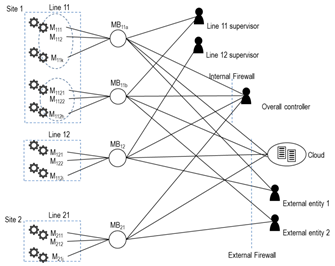
Figure 4 –Architecture with per-line brokers.

In order to guarantee dynamic interoperability across different production lines and industrial sites, and a higher degree of isolation and control over the information flows, a fully distributed IIoT architecture, as depicted in Figure 5, could be also considered [7].

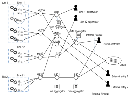
Figure 5 –Distributed architecture with a cascade of brokers.

3.2      E2E data protection

Although both CoAP and MQTT communications can be secured at the transport layer using TLS or DTLS protocol, or at IP layer by IPSec, the presence of intermediate nodes like MQTT brokers or CoAP proxy servers breaks the end-to-end (E2E) security channel. In fact, both (D)TLS and IPsec provide security services only between their end points (i.e. between end systems and the intermediate node), letting the intermediate systems have full control and visibility of the exchanged data. For this reason, E2E security can only be guaranteed under the assumption of a high level of trust at the intermediate node.

Note that although the presence of CoAP proxy server may not be strictly required, it is often used for simplifying network configuration, for flexibility/scalability, and for implementing the publish-subscribe paradigm through the CoAP observe model.

In contrast, in our design we wanted to consider real E2E security, regardless of the level of trust at the intermediate nodes. This requires that data are secured at the application layer directly by the two end systems.

For this purpose, our design includes a security application layer where all exchanged payloads are properly protected in terms of authentication and confidentiality. Figure 6 illustrates an example of a secure exchange of application data between a sensor node (MQTT publisher) and two clients (MQTT subscribers).

Figure 6 –Example of secure exchange of application data between a sensor node (publisher)
and some clients (subscribers).

In particular, when asymmetric encryption is applicable, data authenticity is provided by means of digital signature computed by the source and verified by the recipients. In order to lighten the processing load required to sign and verify data, Elliptic Curve Cryptography (ECC) is preferred in place of RSA or DSA signature. In cases where asymmetric encryption cannot be applicable, data authenticity is provided by means of either: i) message authentication code (MAC), or ii) combined with the encryption, using an authenticated encryption (AE) algorithm.

Data encryption is performed using a symmetric encryption algorithm (e.g. AES-CTR) with a symmetric key that should be generated and managed dynamically (preferred solution). Only in limited cases, with constrained devices where a key management mechanism cannot be applicable (e.g. for very constrained sensors with only sending capability), a long-term symmetric key is directly used for data encryption. In this case, the interactions should be limited to a restricted number of end nodes. In some cases, these nodes may work as adaptors by relaying data to/from the other nodes. The rest of the nodes will consider these adaptors as virtual sources/destinations of the data, and E2E security is provided referring to these nodes as the actual end points.

Considering MQTT as M2M communication protocol, Figure 6 shows the E2E security mechanisms, for protecting either a sensor data m1 published by the device D1 or a command m2 sent by a client C2 for the device D1. In both cases, for simplicity only the distribution of group key (GK) to device D1 is depicted.

3.3      Group key management

To fully support the publish-subscribe paradigm where the same data can be received by multiple endpoints (e.g. MQTT clients subscribing for the same topic), application data has to be encrypted using a symmetric key shared amongst all participants of the communication. The shared key is usually referred to as group key while all participants form the member group. Different communications have different member groups with different group keys. To properly create and share the group key amongst all members, a proper group key distribution mechanism is required. In particular, to efficiently distribute and manage group keys we considered the presence of a Group Key Distribution server (GKD server), usually referred also to as Group Key Distribution Center. The objective of the GKD server is to securely and dynamically exchange the group key with all group members, possibly taking into account the dynamicity of member joins and leaves. To protect these exchanges, the GKD server may use either asymmetric encryption or symmetric encryption, depending on the type of long-term keys shared with the clients. These long-term keys can be: i) the client public key (in this case the GKD server can be configured with either a certification authority certificate used to sign the client certificates, or directly with the client public key), or ii) with al long term secret key associated to the client. In our implementation we considered both cases (client public key and client shared secret key).

Three different group key distribution methods have been considered in our design and are supported in our implementation:

• Static – For each group, a static group key is generated by the GKDC and distributed to each authorized client that requests to join the group.
• Update – For each group, a group key is distributed by the GKDC to all authorized clients. Each time a new client requests to join the group, a new key is generated and distributed to all members of the group (including the previous clients and the new client). Similarly, when a member leaves the group, a new key is generated and distributed to all remaining members.
• Slotted – For each group a dynamic key is considered. Unlike previous methods, the time is now divided in time slots, and for each time slot a different key is used. Such key is automatically derived by the clients from a set of key material received from the GKD server.

3.3.1      Slotted group key management

The slotted GKD mechanism considered in our design and used in our reference implementation is based on the one proposed in [8]. The time axis is divided into time slots, and each time slot has an associated group key. These keys are defined in such a way that only a few data should be maintained and exchanged in order to generate them. In particular, for each group, a root secret key X₀₀ is generated by the GKD server. Starting from this root key, a binary tree can be generated, with the tree leaves representing the slot keys, while all other tree nodes can be used for generating iteratively these slot keys.

If we index with (i,j) the node at depth i and in position j of the binary tree, the root node is the node (0,0), its children are the nodes (1,0) and (1,1), and in general node (i,j) has the children (i+1,2*j) and (i+1,2*j+1). Similarly, each node (i,j),except for the root, has as parent the node (i-1,j/2).

The tree leaves, that are the nodes at depth h, where h is the height of the tree, are the 2^h nodes (h,0), (h,1), …, (h,2^h-1).

Each node (i,j) is associated with key X_i,j. Starting from the root key X₀₀, the two child nodes have the two keys X₁₀ and X₁₁ created from X₀₀ using two one-way functions f₀ and f₁: X₁₀=f₀(X₀₀) and f₁(X₀₀). In general, we have that each node key X_i,j can be used to generate the two child node keys X_i+1,2*j and X_i+1,2*j+1:

X_i+1,2*j = f₀(X_i,j)

X_i+1,2*j+1 = f₁(X_i,j)

In our implementation the functions f₀ and f₁ are simplydefined as:

f₀(X_i,j) = H(X_i,j)

f₁(X_i,j) = H(X_i,j Å 0x01)

where H is the SHA256 hash function.

A tree of height h has at depth h a total number of n=2^h leaves, that correspond to the slot keys K₀=X_h,0, K₁=X_h,1, …, K_n-1=X_h,n-1.

As an example, a tree of height 3, with 8 slot keys, is depicted in Figure 7.

Figure 7 –Slotted group key hierarchy.

The actual height of the key tree will depend on the total number of time slots that has to be managed. For example, with a tree of height 20, it is possible to generate 2²⁰=1 millions of slot keys. If we consider a time slot of 1 hour, we have keys for almost 120 years.

Starting from a node (i,j), it is possible to generate all slot keys that correspond to the leaves of its sub-tree (i.e. the sub-tree with (i,j) as root). These leaves have positions j at depth h of the original tree included in the following range:

[ j*2^h-1 ÷ (j+1)*2^h-1-1 ]

For example, from X_1,0 of the tree in Figure 7 (depth 3) it is possible to generate the keys K₀, k₁, k₂, and K₃, while from X_2,3 it is possible to generate k₆ and K₇.

Focusing on a given slot key K_j=X_h,j, this key can be derived iteratively starting with any node that has the leaf (h,j) as a leaf of its sub-tree. Such nodes are all nodes that are present in the path from the root node (0,0) to (h,j). For example, K2 can be generated starting from X_2,1, X_1,0, or X_0,0.

Each access group has its own key tree. Each time a client joins a group, it should obtain all keys corresponding (only) to the time interval the client is supposed to stay in the group. This guarantees that the client does not have access to data exchanged before or after its membership validity.

The purpose of the key tree is to strongly reduce the key material that has to be sent from the GKD server to a joining client in order to let the client derive the required slot keys. This key material will consist of only a limited subset of node keys that generates all (and only) the slot keys for the requested time interval.

For example, considering the key tree of Figure 7, associated to a group Ga, if a client C1 has to join the group Ga for the interval [0; 5], it will receive from the GKD server the key material {X_1,0, X_2,2}, secured by the GKD server using either the C1 public key K⁺_C1 or the C1 long-term secret key SK_C1. The C1 will use the key X_1,0 to generate K₀, K₁, K₂, K₃ while it will use X_2,2, to generate K₄ and K₅.

Similarly, if client C2 joins the same group for the interval [4; 6], it will receive from the GKD server the key material {X_2,2, K₆}.

This mechanism simplifies the key distribution since keys are distributed only for a given time interval, and no interaction has to be performed by between the GKD server and all previous members when a new member joins, and no action has to be performed when a member leaves at the end of its membership time interval.

In our design, all messages exchanged between the GKD server and clients are performed using MQTT, regardless MQTT is also used as application data exchange.

In the next Section 3.4 we describe how the GKD mechanism is used for managing group keys used for E2E protecting MQTT based application exchanges, while the following Section 3.5 we describe how the GKD mechanism in used by CoAP based application exchanges.

3.4      MQTT extension for E2E security

In this section we define a possible MQTT extension (here called Secure MQTT or SMQTT) to guarantee E2E security to M2M communications based on MQTT protocol.

For this purpose, the data security model described in Section 3.2 and the group key management mechanisms introduced in Section 3.3 are used.

When a client wants to either subscribe to a topic or publish some data to a topic, it first obtains the group key associated to that topic and uses it to handle the E2E security associated to the application payloads for that topic. Without losing generality, let’s assume that the topic coincides with the group id/name. Other cases can easily be considered as a straightforward extension of this case. For example, the same group (i.e. access rights) might be associated to a set of topics, (e.g. same group for all topic names belonging to a topic tree, like “/topic1/#”, or more in general, the same group is associated to distinct topics, like “/topic1” and “/topic2”).

Just to simplify the representation, in the next schemes we consider that the same MQTT broker is used for both the GKD exchanges and application data.

3.4.1      MQTT with STATIC Group Key Distribution

In case the static GKD method is used, for each group one static group key is generated by the GKD server and sent to each client when the client joins the group.

Figure 8 – MQTT with STATIC group key distribution.Figure 8 shows the key distribution protocol.  For simplicity, the MQTT messages used for establishing and maintaining the MQTT connections, and for acknowledgement, have been omitted.

When the GKD server (GKDS) starts, it subscribes to all topics that refer to the key distribution. If the root topic “gkd” is used key distribution, the topic “gkd/#” can be used for this purpose (in MQTT the wildcard “#” can be used to refer to all sub-topics).

Let’s suppose that client C3 has already joined the topic T1, and a group key K0 has been sent to C3. When a new client C1 wants to join the same group for publishing and/or subscribing data for the same topic (or topics) associated to the group, it first subscribes to the key distribution topic “gkd/C1”, then it sends a join request to the GKD server by publishing a JOIN_REQ message to the topic “gkd/1/join”. Here the topic field “1” is used to specify the static method. The JOIN_REQ message contains different parameters including the client identifier and the group identifier.

Figure 8 – MQTT with STATIC group key distribution.

If C1 is authorized to join that group, the GKD server responds to C1 by publishing a JOIN_RESP message to the topic “gkd/C1”. The JOIN_RESP message contains, amongst other parameters, the group identifier, and the group key (K0). The payload of the JOIN_RESP message is secured (authenticated and encrypted) using the long-term key(s) shared between the GKD server and C1 (the private key of GKD server and the public key of C1 in case public-key cryptography is used, or the long-term secret key associated to C1).

When C1 receives this response, it can subscribe to topic T1 and start receiving or sending (publishing) data to this topic.

Once a new client C2 wants to join the same group, the same procedure is executed and the same group key K0 is exchanged.

3.4.2      MQTT with UPDATE Group Key Distribution

Figure 8 – MQTT with STATIC group key distribution.Figure 9 shows the key distribution protocol for the update GKD method. Similar to the previous case, when started, GKDS subscribes to the general GKD topic “gkd/#”. Now suppose that C3 has already joined the group and a group key K0 has been distributed. When client C1 wants to join the same group, it subscribes to topic “gkd/C1” and sends a JOIN_REQ message to topic “gkd/3/join”; the topic field “3” indicates the update method.

Figure 9 – MQTT with UPDATE group key distribution.

If C1 is authorized to join that group, the GKD server adds C1 to the list of group members, generates a new group key K1, and sends it to all group members (in this example only C3 and C1). This is done by separately publishing JOIN_REQ messages (used as key update messages) to the proper topics corresponding to the different members. C1 also subscribes to topic T1.

When the group members receive the new key, they can start using it.

If the client C2 wants later to join the same group, the same procedure is executed, and a new group key (K2) is generated and distributed, as shown in Figure 9.

3.4.3      MQTT with SLOTTED Group Key Distribution

Figure 8 – MQTT with STATIC group key distribution.In case the slotted GKD method is used, the GKD server generates a root key for each requested group, and uses it for generating the proper key material that can be used by the joining clients to derive all slot keys referring to (and only to) all time slots the clients requested and have been authorized for.

In Figure 10Figure 9 an example of message exchange with the slotted GKD method is shown. In this scheme, fields t:TI1, and t:TI2, in the JOIN_REQ and JOIN_RESP messages specify the time interval requested by the clients (JOIN_REQ) and authorized by the server (JOIN_RESP), for which the proper key material KM1 and KM2 are exchanged. Topic field “3” indicates the slotted method.

In the scheme, SK_i and SK_j are two slot keys referring to two different time slots i and i.

Figure 10 – MQTT with SLOTTED group key distribution.

3.5      CoAP extension for E2E security

The same GKD methods can be easily used with CoAP for dynamically generating and distributing secret keys used to secure E2E application data exchanges.

In Figure 11 an example of protocol exchange for setting-up group keys for two CoAP clients (C1 and C2) and a CoAP server (S1) is shown. In this scheme, we consider that server S1 already joined the group res1. The identifier res1 can be any identifier that is associated with a set of resources (in some practical cases can be also a resource path or just the server’s name). In this example, for simplicity we used “res1” as the name for the group (topic) and for the name of a target resource.

When started, server S1 requests keys for all its resources by joining one or more groups. In the example S1 we suppose that S1 already joined the group that res1 is associated with.

If a client C1 wants to access res1 it first requests to join the group for res1. In the figure we supposed that the update GKD method is used, and, in accordance with this method, a new group key K1 is generated and sent to all group members, including the new client C1 (in this case just S1 and C1). When C1 receives the new key, it can send for example a CoAP GET request to S1.  In case of success, S1 sends a 2.05 Content response to C1, by protecting the payload using key K1.

If later a new client C2 wants to access the same resource, in accordance with the previous procedure, a new key K2 is generated by the GKD server and distributed to all group members. Client C2 (or C1) then uses this key to securely exchange a CoAP payload with S1 (e.g. for getting the resource res1 or putting a new value).

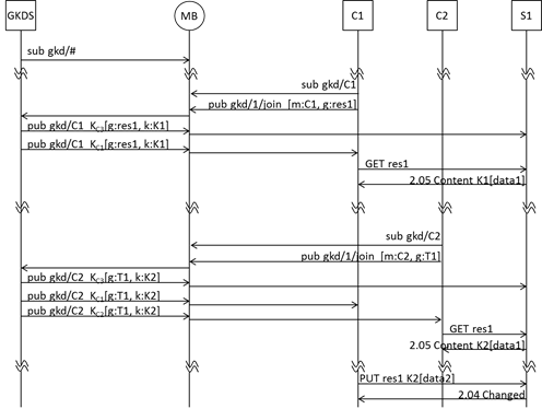
Figure 11 –CoAP with UPDATE group key distribution.

3.6      Implementation

All the mechanisms and protocols described in the previous sections 3.1, 3.2, 3.3, 3.4, and 3.5 have been implemented and tested. The reason for this was twofold: first, to demonstrate their correctness and feasibility, and second, to provide a reference implementation.

The source code, libraries, and documentation can be found at:
https://github.com/serics-assist/e2e-security

3.6.1      KD Server

The GKD server has been implemented in Java.  All three GKD methods (static, update, and slotted) have been implemented. For MQTT communications the Eclipse Paho[1] [2] library has been used.

The server can be run on a Java 10+ JVM and supports different options at command-line that can be shown using the ‘-h’ option.  It just requires a standard MQTT (e.g. Eclipse mosquitto[3]) running and reachable at a given IP address.

3.6.2      Secure MQTT

The MQTT extension with E2E security described in section 3.4 has been implemented. Different implementations are available in Java, Python, and C programming languages.

In particular, the C implementation of a Secure MQTT client is available for standard PC (compiled with GNU GCC) and for Arduino devices.

The reference implementation is the Java one, that supports all three GKD methods (static, update, and slotted).

For this reference implementation we used the the Eclipse Paho[4] [5] library for MQTT support.  However, in order to let our Secure MQTT implementation be independent from the actual MQTT library that is used, a new Java MQTT API has been defined (through the interface io.ipstack.mqtt.MqttClient). The Secure MQTT client (assist.smqtt.SecureMqttClient) is provided as an implementation of this interface.

This implementation can be easily tested by launching the test.GKDMqttTest program that runs a GKD server and n SecureMQTT clients. One of the three GKD methods can be selected.  By default, it expects a standard MQTT running locally at 127.0.0.1:1883, however it can be properly configured, using the ‘-b’ option, to use an external broker.

3.6.3      Secure CoAP

The CoAP extension with E2E security described in section 3.5 has been also implemented. This reference implementation is in Java and includes its own CoAP library, so no external third party CoAP library is needed.

In particular, the SecureCoAP implementation is provided though both a SecureCoAP client (assist.scoap.SecureCoapClient) and a SecureCoAP server (assist.scoap.SecureCoapServer), as extensions of CoAP client (io.ipstack.coap.client.CoapClient) and CoAP server (io.ipstack.coap.server.CoapServer), respectively.

This implementation can be tested by launching the test.GKDMqttTest program that runs a GKD server, a SecureCoAP server S1, and a SecureCoAP client C1. When started, the server S1 obtains a group key for a resource (“/test”) that it owns.

When the client starts, it wants to GET the “/test” resource from server S1. For this purpose, it first requests a valid group key for such resource, then it gets the resource (GET /test) from the CoAP server, secured using the corresponding group key.  By default, this program expects a standard MQTT running locally at 127.0.0.1:1883, however it can be configured to use an external broker.

3.6.4      Embedded devices

The SecureMQTT protocol has been also implemented and tested on embedded devices (currently using Arduino Nano 33 IoT boards).

We implemented SecureMQTT as extensions of both the standard MQTT (that runs over TCP) and MQTT-SN.  MQTT-SN (MQTT for Sensor Networks) [6] is the porting of MQTT that runs over UDP; it is lighter than MQTT and is suitable for very constrained devices and/or for environments where TCP is either inefficient or unusable.

In order to run SecureMQTT with MQTT-SN, a standard MQTT broker can be used (e.g. mosquitto) together with a MQTT-SN gateway (e.g. Eclipse Paho MQTT-SN Transparent Gateway[6]).

4       Anomaly detection

4.1      Anomaly detection in IIoT

Anomaly detection is a fundamental component in ensuring the reliability and integrity of exchanged messages and application data, particularly when the information originates from untrusted external sources or is transmitted over unsecured communication channels. In such contexts, data may be subject to disruption, manipulation, or substitution by unauthorized or malicious actors. Within this report, an “anomaly” is defined as any deviation from established or expected normal behavior.

In network traffic, anomalies can stem from deliberate actions by adversaries, including:

• cyberattacks exploiting vulnerabilities in device hardware, firmware, or software update mechanisms;
• attacks targeting communication channels at the physical or logical layers (e.g., data-link or network layers);
• tampering with message content, especially in scenarios lacking end-to-end security, where intermediate nodes may be compromised (see Deliverable D2 for further discussion).

In contrast, anomalies in sensor data may result from either malicious interference or non-malicious factors such as:

• device or system faults, including hardware/software failures, sensor calibration errors, or power issues (e.g., low battery levels);
• communication disruptions caused by interference or intermittent connectivity;
• environmental influences such as external noise or unpredictable physical events.

These anomalies may present as: i) short-term irregularities, such as outliers, noise spikes, or reduced measurement precision, or ii) long-term deviations, including signal drifts, persistent offsets, or stuck-at values.

Detection of anomalies in IIoT systems introduces several technical challenges such as i) resource limitations on edge devices, including constraints in processing power, memory, and energy; ii) complex data characteristics, like high volume, noise, and non-stationarity.

The primary objective of anomaly detection is to enable early identification of faults or security incidents, thereby preserving system and data integrity and enhancing the trustworthiness and operational efficiency of the overall infrastructure.

Common approaches to anomaly detection include both statistical techniques and machine learning-based models, such as Principal Component Analysis (PCA), Multiscale PCA (MSPCA), Autoencoders, and Recurrent Neural Networks (RNNs). These methods aim to model normal system behavior and identify significant deviations.

4.2      Goal and functional description

The goal of this component is to support robust detection of anomalies on exchanged and collected data, within IIoT environments.

The first step is to acquire and process time-series data from relevant industrial sources. Whenever possible, real-world IIoT datasets are incorporated to establish a baseline of normal system behavior. This foundation enables more realistic modeling and ensures that subsequent experiments reflect operational conditions.

Different key anomalies and attack types have been defined to represent the range of disturbances under investigation.

Due to the limited availability of large datasets containing both correct and wrong IIoT data, synthetic anomalies have been generated and injected into nominal data streams. This methodology enabled systematic evaluation of model robustness under diverse and well-characterized conditions.

Time-series data are segmented into fixed-length windows to support both temporal and statistical analyses. From each segment, descriptive statistical features (including mean, standard deviation, skewness, and kurtosis) are extracted for feature-based modeling. Balanced datasets comprising normal and anomalous instances are constructed and formatted to accommodate the requirements of both deep learning and traditional machine learning models.

The framework supports multiple learning paradigms for anomaly detection. Binary classification models are employed to distinguish between normal and anomalous states, with optional extension to multiclass classification for specific anomaly types. Architectures capable of processing raw time-series inputs (e.g., CNN, LSTM, TCN) can operate in parallel with models leveraging statistical feature vectors, enabling cross-model comparisons.

Models are trained using hybrid datasets that integrate real and synthetically generated samples. Performance is quantified through standard classification metrics, including Accuracy, Precision, Recall, F1-Score, and Confusion Matrix analysis. Validation on independent datasets ensures that findings generalize beyond the initial training domain, enhancing confidence in real-world applicability.

Post-training analyses examine model performance across architectures and data representations to identify the most effective approaches for specific sensor modalities and anomaly characteristics. These comparative insights elucidate trade-offs between complexity, accuracy, and interpretability, informing model selection for operational deployment and further development.

4.2.1      Functional description

These have been the main design aspects:

1. Synthetic anomaly generation: a core design choice is the reliance on synthetically generated anomalies based on predefined mathematical models. This is necessary due to the likely scarcity of real-world, labeled anomaly data. It provides a controlled way to create varied and balanced datasets.
2. Dual data representation: The system is designed to process and feed data to machine learning models in two distinct formats:
   • Raw temporal sequences: Using fixed-length windows of sensor readings directly.
   • Extracted statistical features: a few statistical features (mean, std dev, skewness, kurtosis, etc.) are computed from these temporal windows. This allows for evaluating which representation works better for different models and data characteristics.
3. Comparative framework: the entire design facilitates a systematic comparison of different machine learning approaches (time-series deep learning vs. feature-based ensemble/automated methods) on the same defined tasks (anomaly types) and datasets.
4. Feature engineering for robustness: for feature-based models, the selection of statistical features (mean, std dev, skewness, kurtosis, median, mode) is a key design aspect aimed at capturing deviations in the input data distribution and shape, potentially making detection more robust than just looking at raw values.
5. Modularity: the process is implicitly modular: data sourcing, anomaly generation, dataset creation, feature extraction, model training, and evaluation are distinct logical steps.

The developed anomaly detection component can be functionally divided into the following subcomponents:

1. Data Source interface:
   • Subcomponent role: this module is responsible for loading and initially processing the available datasets.
   • Relationships: it provides baseline normal time-series data to the Dataset Constructor.
2. Anomaly Generator:
   • Subcomponent role: the module will support different anomaly types.
   • Relationships: Generates synthetic anomaly dataset on requests. Provides these generated anomalies to the Dataset Constructor.
3. Dataset Constructor:
   • Subcomponent role: the module takes normal data from the Data Source and synthetic anomalies from the Anomaly Generator. It segments the data into fixed-length windows. It combines normal and anomalous windows to create labeled datasets (e.g., normal=0, anomaly=1) suitable for training, validation, and testing. Finally, it ensures balancing between normal and anomalous samples.
   • Relationships: Receives data from Data Source and Anomaly Generator. Outputs labeled data windows to the Feature Extractor and directly to the Time-Series Model Training Pipeline.
4. Feature Extractor:
   • Subcomponent role: the model calculates predefined statistical features (Mean, Std Dev, Skewness, Kurtosis, Median, Mode) for each data window provided by the Dataset Constructor.
   • Relationships: Receives labeled data windows from the Dataset Constructor. Outputs labeled feature vectors to the Feature-Based Model Training Pipeline.
5. Machine Learning Model Pipelines:
   • Subcomponent 1: Time-Series Models (CNN, LSTM, TCN): Takes labeled, raw temporal windows as input. Contains the logic for defining and training the models.
   • Subcomponent 2: Feature-Based Models (XGBoost, AutoGluon): Takes labeled feature vectors as input. Contains the logic for training these models (using libraries like XGBoost and AutoGluon).
   • Both pipelines receive their respective data formats from the Dataset Constructor or Feature Extractor. They eventually produce trained models.
6. Model Evaluator:
   • The module takes a trained model (from either pipeline) and a labeled test dataset (in the appropriate format – sequence or features). It runs predictions and calculates performance metrics (Accuracy, Precision, Recall, F1-Score, Confusion Matrix).
   • Receives trained models from the ML pipelines and test data. It outputs performance metrics.
7. Results Analyzer:
   • The module is totally or partially automated to collect and compare the performance metrics from the Model Evaluator across different models, anomaly types, and data representations. Finally, it generates summary graphs and conclusions.
   • Receives performance metrics from the Model Evaluator.

4.3      Implementation

In our implementation, for the training and testing phases real-world sensor data from freely available public dataset have been used. In particular, for the experiments, we used a dataset containing three measurements from environmental sensors: i) CO2 levels (ranging around 2000 ppm), ii) Temperature (approximately 19-23°C), iii) Humidity (around 38%).

The training dataset comprises 8143 samples collected at one-minute intervals over two days, with additional validation and test datasets containing 9752 and 2665 samples respectively.

To overcome the lack of availability of large datasets that combine both benign and anomalous data, we generated synthetic anomalies based on mathematical models. We used the same approach used in [9].  We created six distinct anomaly types, classified into two categories: long-term and short-term anomalies.

To cover the different types of anomalies, we used the following simple model. Let x be the vector of normal data, and y the vector of data with anomalies, y is generated as follows:

𝒚=𝐴𝒙+𝐵𝝍+𝐶𝝓

where 𝝍 represents a long-term offset vector, i.e., the term that gives rise to long-term anomalies, while 𝝓 denotes the short-term offset vector, i.e., the term that gives rise to short-term anomalies. The elements of this model are independent and identically distributed random variables that follow the distribution of a given short-term anomaly. A, B, and C are coefficients used to form a given anomalous shape, and they assume values 0 or 1.

As long-term anomalies, we considered the following types:

1. : Signal remains fixed at a constant value
2. : Systematic shift in signal baseline
3. : Exponential signal degradation over time

As short-term anomalies we considered:

• : Gaussian noise corruption
• : Isolated extreme values
• : Brief bursts of abnormal values

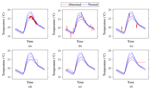
Figure 12 – The six considered forms of anomalies (from[9]).
Short-term: (a) Precision degradation. (b) Outlier. (c) Spike. Long-term: (d) Stuck-at. (e) Offset. (f) Drift.

The source code and documentation can be found at:
https://github.com/serics-assist/anomaly-detection

4.3.1      Data Preprocessing and Feature Engineering

The system implements a dual-representation approach:

Temporal Windowing – Data divided into 20-sample windows (1200 seconds each) – Preserves local temporal patterns – Prevents anomalies from spanning multiple windows

Statistical Feature Extraction – For each temporal window, six statistical features are computed:

This dual representation enables different machine learning models to leverage either temporal sequences or statistical summaries, depending on their architectural strengths.

4.3.2      Machine Learning Models

The system implements five distinct machine learning architectures, strategically chosen to exploit different data representations.

Temporal Sequence Models:

Feature-Based Models:

• [7] – Ensemble of decision trees – Iterative error correction through gradient boosting – Built-in regularization to prevent overfitting – Efficient parallel processing – Handles missing values automatically – Provides feature importance rankings
  • [8] – Automated machine learning (AutoML) framework – Ensemble of multiple models – Automatic hyperparameter optimization – Minimal code requirements – Consistently outperforms single models – Preset configurations for quality optimization

4.4      Experimental Results

Since we used synthetically generated anomalous data, we have studied how intense these anomalies must be for our system to detect them with high accuracy. We considered a target accuracy of 95%, with the 68-95-99.7 rule (a weel-known empirical rule that describes how data are distributed in a normal distribution), providing a statistically sound confidence level for critical applications.

The balanced dataset approach ensures equal representation of normal and anomalous samples (50/50 split) to prevent model bias.

Analyzing the results, the feature-based models show an accuracy of around 96%, while the time-interval-based models stand around 92.42%.

Feature-based models (AutoGluon, XGBoost) consistently outperformed temporal models (CNN, LSTM, TCN) by 2-4 percentage points for CO2 data, due to high signal variance enabling effective statistical feature extraction.

In Figure 13, the accuracy of models based on time intervals or statistical features versus different types of anomalies on CO2 dataset are plotted.

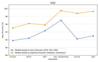
Figure 13 – CO2: Comparison of model accuracy vs. different types of anomalies.

Similarly, in Figure 13 and Figure 15 the accuracy of models based on time intervals or statistical features versus different types of anomalies are plotted, in the cases of temperature and humidity datasets.

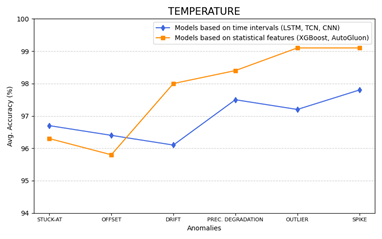
Figure 14 – Temperature: Comparison of model accuracy vs. different types of anomalies.

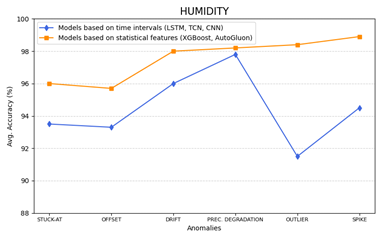
Figure 15 – Humidity: Comparison of model accuracy vs. different types of anomalies.

4.4.1       Cross-Validation on Independent Dataset

In order to verify generalizability, the system was also tested using a different dataset (Intel Berkeley Research Lab dataset, 2004)[9], comprising about 2.3M values of data collected from 54 temperature, humidity, light, and voltage sensors.

Figure 16 summarizes the comparison of the anomaly detection accuracy with the original dataset and the Intel dataset, versus the different types of considered anomalies.

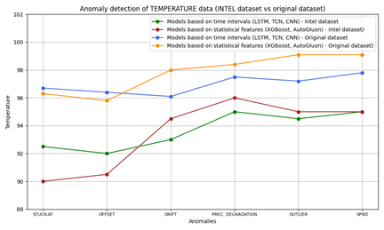
Figure 16 – Cross-validation on independent data.

The demonstrated transferability of detection approaches across different sensor deployments, evidenced by successful validation on the Intel dataset, suggests that the developed methodology generalizes beyond the specific experimental context. The convergence of optimal parameter settings with those reported in prior literature, despite different datasets and geographic contexts, further supports the robustness and reproducibility of the approach. This generalization provides confidence that the techniques can be adapted to different IIoT deployments through systematic parameter tuning based on local signal statistics rather than requiring complete re-engineering.

5       Source Code Vulnerability Detection

5.1      Context and Goals

Detecting vulnerabilities in source code is vital to prevent exploitation, unauthorized access, and system disruptions.  Proactive identification and remediation of such vulnerabilities are essential to mitigate exploitation risks, reduce operational downtime, protect proprietary assets, and strengthen overall system resilience.

However, the escalating scale and structural complexity of modern software systems makes conventional, manually driven detection techniques increasingly impractical.  Consequently, automated approaches—particularly those grounded in machine learning —are emerging as promising alternatives.

Recent advancements in deep learning and large language models have demonstrated strong potential to generalize from known vulnerability patterns, adapt to evolving codebases, and operate effectively across extensive and heterogeneous datasets.

In contrast to rule-based or signature-driven systems, ML-based methods can autonomously uncover subtle, previously unseen vulnerability patterns through data-driven learning, positioning them as a compelling solution for contemporary secure software engineering.

Unfortunately, currently available LLM models, trained solely on raw source code text, are not sufficient to correctly detect software vulnerabilities.  For this reason, our primary objective was to improve the capability to accurately detect software vulnerabilities.  In order to overcome the deficiency of LLMs in capturing the syntactic and semantic structures of code, the proposed detection component incorporates graph-based representations—such as Abstract Syntax Trees (ASTs), Program Dependence Graphs (PDGs), and Control Flow Graphs (CFGs)—which are further unified into a Code Property Graph (CPG) to enrich the model’s contextual understanding.

In addition, the proposed systems aims to exploit: i) in-context learning to inject domain-specific knowledge and relevant vulnerability patterns directly into the LLM through curated example demonstrations, thereby enhancing its reasoning and generalization capabilities; ii) an effective retrieval mechanism for selecting the most relevant code demonstrations based on multi-dimensional similarity metrics—encompassing semantic, lexical, and syntactic similarities—to the target code under analysis.

5.1.1  Functional description

The main functional aspects of this component are:

1. Vulnerability detection: the system analyzes input source code (specifically C/C++ in the evaluated context) at a specified granularity (e.g. function level) and classifies it as either ‘Vulnerable’ or ‘Non-vulnerable’.
   Optionally, the system would provide advanced classification on the vulnerable code, like information on the CWE, if identified.
2. LLM integration: the system utilizes one or multiple Large Language Models as its core engine for analysis and prediction. 
3. Graph structure generation: the system will generate a Code Property Graph (CPG) representation of the input source code, combining Abstract Syntax Tree (AST), Program Dependence Graph (PDG), and Control Flow Graph (CFG) information (using a tool like Joern). 
4. Graph information extraction: the system extracts relevant structural and semantic information from the generated CPG to be used as input for the LLM. This includes representations of nodes (e.g., statement types, identifiers), edges (e.g., control flow, data flow), and pertinent attributes that can inform the LLM.
5. Demonstration selection: the system implements a mechanism to select a relevant demonstration (a similar code example with its known vulnerability status) from a candidate pool based on (but not limited to) a combination of Semantic similarity (e.g., using code embeddings like CodeT5), Lexical similarity (e.g., based on token sets) and Syntactic similarity (e.g., based on AST).
6. Prompt engineering: the system constructs a structured prompt for the LLM that includes some key elements such as: i) the target code snippet to be analyzed; ii) specific instructions for the vulnerability detection task; this includes the objective of the LLM, including the desired output format, which ensures reliable parsing of model responses; iii) the extracted graph structural information (nodes and edges); iv) the selected demonstration examples and their label (for in-context learning).
7. Output Parsing: the system must be able to parse the LLM’s output to extract the final binary classification (‘Vulnerable’/’Non-vulnerable’).

5.1.2  Component Design

Most Significant Design Aspects:

1. Hybrid Information Fusion: The core idea is not to rely solely on the LLM’s inherent understanding of code (as plain text) but to explicitly augment it with structured information. This detection component fuses: 
2. Code Semantics/Lexical Info (via LLM & Embeddings): Leverages the LLM’s pre-trained knowledge and uses embeddings (like CodeT5) for semantic similarity. 
3. Code Syntactic/Structural Info (via Graphs): Explicitly generates and inputs Code Property Graph (CPG) data (nodes, edges representing AST, CFG, PDG) to provide structural context the LLM might otherwise miss. 
4. Domain-Specific Examples (via In-Context Learning): Provides carefully selected, relevant examples (demonstrations) directly within the prompt to guide the LLM’s reasoning specifically for the vulnerability detection task. 
5. In-context Demonstration Retrieval: Instead of random or simple example selection for in-context learning, our detection component employs a multi-faceted retrieval strategy. It selects demonstrations based on a combined measure of similarity across: 
6. Semantic Similarity: Using code embeddings to find conceptually similar code. 
7. Lexical Similarity: Comparing token sets. 
8. Syntactic Similarity: Comparing AST structures. 

This aims to provide the LLM with the most contextually relevant positive or negative examples, significantly boosting learning effectiveness. 

3. Structured Prompt Engineering: The system doesn’t just feed raw data. It carefully constructs a detailed prompt for the LLM, incorporating: 
4. The target code snippet. 
5. Task instructions (including role priming and domain specification: “You are an excellent programmer doing C/C++ vulnerability detection”). 
6. The extracted graph structure information (nodes and edges list). 
7. The retrieved demonstration code snippet and its corresponding label (vulnerable/non-vulnerable). Optionally, vulnerability information and relative inference approach. This structured input is crucial for guiding the LLM effectively.

Subcomponents and their relationships: 

Based on Figure 17 and the text, the overall detection component consists of three main modules, plus the core LLM engine: 

1. Demonstration Selection Module (Figure 18): 
2. Function: Identifies and retrieves the most relevant code example (demonstration) from a pool of candidate code snippets to be used for in-context learning. 
3. Inputs: Target Source Code, Candidate Code Pool (with labels). 
4. Process: 
5. Calculates semantic similarity (using CodeT5 embeddings and T-SNE/L2 distance) to filter candidates. 
6. Calculates lexical similarity (token set comparison). 
7. Calculates syntactic similarity (using Joern for ASTs and SimSBT for tree traversal/edit distance). 
8. Combines lexical and syntactic similarity using a mixed score to select the top demonstration from the semantically similar candidates. For the score, different approaches are considered (e.g., a weighted sum, a heuristic, or a small learning model) the specifics of which will be subject to empirical tuning.
9. Output: The selected Demonstration (code snippet + vulnerability label). 
10. Graph Structure Information Generation Module (Figure 19): 
11. Function: Generates a structured representation (CPG) of the target source code, capturing its syntactic and semantic structure. 
12. Inputs: Target Source Code. 
13. Process: Uses a tool like Joern to parse the code and create a Code Property Graph (CPG), which integrates AST, PDG, and CFG. Extracts lists of nodes and edges with their types/attributes. 
14. Output: Graph Structured Data (List of Nodes, List of Edges). 
15. Prompt Optimizer Module (Figure 20): 
16. Function: Automate selection of most effective prompt layout and elements, dealing with general setup constraints, Target Code characteristics and specific candidate CWE (if any).
17. Inputs:
18. Target Source Code. 
19. Graph Structured Data (from Module 2)
20. Selected Demonstration (from Module 1)
21. Process:
22. Assemble the final prompt by selecting and combining the basic instruction of identity/domain information, the target code snippet, the graph node/edge information, and the selected demonstration with its label.
23. May select a different prompt approach (e.g., Cot) and layout (e.g., provide specific CWE example, or a pair of vulnerable and non-vulnerable similar code) based on heuristics or limitations
24. Sends the prompt to the Enhanced Vulnerability Detection Module.
25. Output:  Tailored textual prompt
26. Enhanced Vulnerability Detection Module (Figure 21): 
27. Function: Orchestrates the process, receives the final prompt, interacts with the LLM(s), and produces the final prediction. 
28. Inputs: 
29. Tailored textual prompt
30. Process: 
31. Adapt the prompt if needed by specific LLM constraints
32. Sends the complete, structured prompt to the LLM. 
33. Receives the raw textual prediction from the LLM.
34. Optionally, it can perform multiple passes with different LLMs, based on constraints.
35. Output: Vulnerability Prediction (‘Vulnerable’ or ‘Non-vulnerable’).

Relationships: 

• Modules 1 and 2 operate largely in parallel, both taking the Target Source Code as input (Module 1 also needs the candidate pool). 
• Module 3 is dependent on the outputs of both Module 1 (Selected Demonstration) and Module 2 (Graph Structured Data). 
• Module 3 integrates these inputs along with the original code and predefined prompt components to create the final input for the LLM. 
• Module 4 takes the desired custom final prompt, but being still able to modify it based on specific constraints (e.g. reduced context window).
• The main reasoning engine is at least one instance of LLM. This acts as the main reasoning engine, taking the structured prompt from Module 4 and producing the raw prediction, which Module 4 then interprets as the final output.
• Optionally, in Module 4, if the context allows (e.g., available resources), additional models can be used to improve the final detection, for example by comparing their outputs.

The diagram in Figure 17igure 17 illustrates the overall data flow and interaction between the main modules.

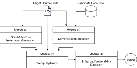
Figure 177 – Overall data flow and interaction between the main modules

The Input Source Code is fed into both the Demonstration Selection (Module 1) and theGraph Structure Information Generation (Module 2), which operate concurrently, and into the Prompt Optimizer (Module 3).

The Demonstration Selection module accesses a Candidate Code Pool to retrieve relevant examples. The outputs from Module 1 and Module 2 are then passed to the Prompt Optimizer (Module 3), that is followed by the Enhanced Vulnerability Detection (Module 4). Within this module, the LLM Engine is accessed. The LLM processes the prompt and returns a raw textual prediction, which is parsed to produce the final ‘Vulnerable’/‘Non-vulnerable’ output (and optionally, explanations or repair attempts).

The general design of each module is reported in Figure 18, Figure 19, Figure 20, and Figure 21.

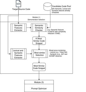
Figure 18 – Demonstration Selection module(1)

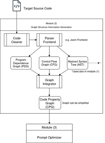
Figure 19 – Graph Structure Information Generation module (2)

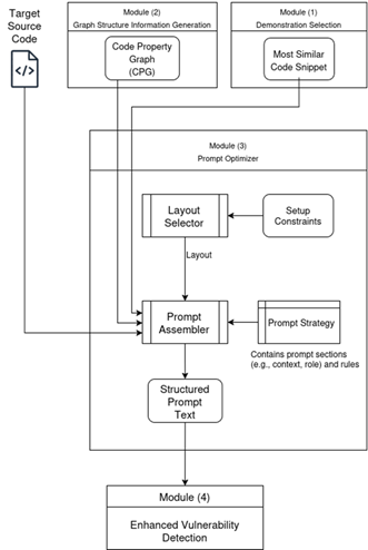
Figure 20 – Prompt Optimizer module (3)

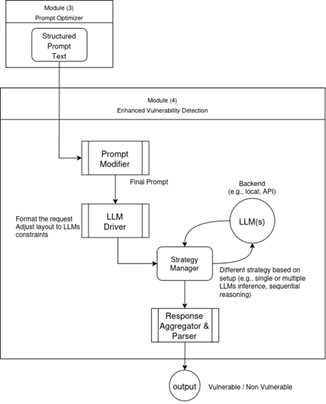
Figure 21 – Enhanced Vulnerability Detection module (4)

5.2      Implementation

This section presents a discussion of the implementation of the Software Vulnerability Assessment solution (called also system or tool).  It focuses on the technical aspects comprising data structures and algorithms employed, as well as the logical formulations, including aggregation strategies, that underpin the system’s operational framework.

Design details, core components, and execution workflows that collectively realize the vulnerability detection functionalities are also presented.

The source code and documentation can be found at:
https://github.com/serics-assist/vulnerability-detection

5.2.1      Overview

The developed system is the result of research and experimental oriented development, currently intended for testing and prototyping contexts. However, it is designed to be easily interpreted and extended, allowing future enhancements (especially regarding usability, user experience) and feature integration (more comprehensive workflow) toward a fully functional vulnerability assessment tool-chain, integrating code graphs and LLM-based reasoning.

The development follows an incremental and modular approach.  The system that can ingest code snippets – primarily designed to work at “function” granularity – and produces structured vulnerability classification outputs.

The implementation supports both offline experimentation on labeled state-of-the-art datasets, and integration with external or manually provided code snippets.

5.2.1.1      Design and Implementation Objectives

The main objectives considered during implementation are the following:

• Maintain a clear and organized codebase structure, to facilitate consultation, reproducibility, and modification.
• Ensure abstraction from specific data source and LLM models/provider, allowing scalability to future use additional languages ​​and LLM models.
• Use standard interfaces and API specifications to improve modularity and interoperability.
• Facilitate deployment through containerization
• Enable flexible and simple configuration through external files, like YAML or JSON.

5.2.1.2      System Architecture

The system demonstrates a modular and extensible architecture, supporting diverse ML and code-analysis backends through standard or easily integration.

Main operations concerns are clearly separated by different file, regarding:

• Pre-processing: dataset loading, cleaning, code embeddings generation.
• Main Execution – Vulnerability detection: functional modules that perform prompt construction, reasoning, and classification.
• Post-processing: results and performance evaluations, metrics, and file savings.

Other subdivisions are identified by the distinction between modules and sub-operations, such as embedding generation, feature extraction, or model interaction.

5.2.1.3      Configuration and Deploy

The system uses external configuration files to manage parameters such as model endpoints, dataset paths, embedding dimensions, and classification thresholds.
This structure abstracts the operational logic from the implementation, facilitating adaptation to new APIs, datasets, or model architectures.

Containerization through Docker allows consistent testing and reproducibility across environments.

5.2.1.4      Algorithmic Components Development

The development followed an incremental cycle. Each component was first validated through individual tests to ensure stable integration.

The system has been tested on multiple labeled datasets for software vulnerability research, especially publicly available code collections.

Moreover, different LLM models and providers have been considered and used.

Alternative approaches were designed, tested, and implemented, primarily regarding Prompt Engineering and Vulnerability Detection, which can be activated alternatively through a few lines of configuration code.

These are better explained in the following sections.

5.2.2      Technology Stack and Tooling

The system is primarily implemented in Python 3, using built-in methods where possible, and including external libraries (like Networkx, Pandas, Pytorch) to support key functionalities. External tools are integrated by wrapper or system calls.
Deployment and workflow orchestration utilize additional technologies such as Docker, shell scripting, and configuration files.

The main components of the technology stack are summarized here:

• Joern, for the generation and interaction with graphs like CPG and AST.
• Clang-Formatter, for consistent source code parsing and formatting.
• CodeT5 Model, for code embedding and representation learning.
• LLMs, via different interfaces. The system can interact with multiple LLM backends, including locally hosted open-source models (using Llama) and remote API-based providers (Gemini, OpenRouter).
• Data Management. Intermediate and persistent data is managed using formats like XML and JSON, for serialization, interchange, and storage of code artifacts, model outputs, and configuration states.
• Docker and Docker Compose are employed for the definition, orchestration, and deployment of system components.

5.2.3      Module-wise Implementation Details

For each module described in Section 5.1.2 the following outlines the implementation logic and technical integration, reflecting the established data flow between system components.

The description is presented as the system operates on a batch of labeled data, but can easily be extended to match alternative formats such as real-time streaming.

To properly work, the system needs a trusty labeled pool of data, referenced as “known functions” dataset, required especially for similarity-based code selection. This pool is used as a structured and queryable collection, from which relevant samples are extracted using selection logic within the Demonstration Selection Module, and incorporated to help the LLM in the pattern matching process. To ensure the similarities selection to be effective, the known function requires characteristics, such as language and domain of use, to be very close to the input function we wish to assess for vulnerability – also called “object function”.

5.2.3.1         Demonstration Selection (Module 1)

The first module interfaces with both the input functions—code segments to be analyzed—and the known functions stored in one or more pre-labeled datasets.  Dataset access is managed through a dedicated Python class that abstracts the handling of different dataset formats. The class exposes a unified interface for loading, parsing, and normalizing input data, while supporting implementation-specific subclasses for dataset-specific procedures.  Each reader method encapsulates the parsing logic (interface) appropriate to its dataset format or structured archives.

The processed output is returned as a pandas DataFrame containing at least two core fields: a source code snippet and its corresponding label (vulnerable / non vulnerable).

Pre-processing

The first step is to perform, on each record in the dataset, a cleaning procedure, and to generate the related semantic embedded features in advance (they are very time consuming) to be more efficient in the next modules.

Data cleaning and Embedding generation are done for each code snippet in the known function dataset.

Data cleaning consists of a data verification (check if label is correctly present, function is well formed, etc) and a normalization process, executed using the clang-format system utility, which enforces a deterministic source layout across all code samples. This procedure standardizes indentation, spacing, preprocessor directive ordering, and line length. The configuration applies the LLVM style definition, consistent with established LLVM coding conventions.

Next, the tool proceeds on embedding generation. The code snippet is partitioned into multiple chunks to comply with the maximum context size supported by the downstream model. Each chunk corresponds to a substring of the original code, limited to a maximum length of N characters. This segmentation preserves local syntactic and semantic coherence while permitting independent embedding of code portions that exceed model constraints. For each chunk, tokenization and embedding computation proceed through the following steps:

• Tokenization: The tokenizer associated with the selected model converts textual code representations into discrete tokens.
• Tensor Conversion: The tokens are converted into Pytorch tensors and transferred to the active computing device, using a CUDA-enabled GPU when available.
• Embedding Generation: The embedding model processes the tokenized sequences to extract high-dimensional semantic features, producing vector representations as NumPy arrays.
• Aggregation: All chunk-level embeddings derived from the same snippet are aggregated to form a unified representation. A simple mean-pooling operation is applied, computing the element-wise average of all chunk vectors to obtain a single, fixed-size embedding for the complete snippet.

The implementation is tested using the codet5p-110m-embedding model as the reference embedding generator, employing its tokenizer configuration and pre-trained encoder, using a length N = 512 characters.

The entire embedding pipeline supports parallel execution.

As output, pre-processing produces a dataset stored in shared file-system storage. Each record contains a normalized code snippet, its corresponding semantic embedding, and associated metadata such as label.
The embedded dataset is serialized in JSON or JSONL format, ensuring compatibility with subsequent modules and experimental workflows.

Following this, for experimentation purposes, the dataset can be partitioned into two subsets according to a predefined ratio (like 80/20). The first subset forms the support pool used to retrieve similar functions during analysis (the known functions) and prompt construction. The second subset is reserved for evaluation, supplying the input functions selected for vulnerability assessment.

Main Execution

The Main Execution is performed on every input function, iteratively as they arrive.
At this stage, the system orchestrates sequential invocations of the lexical, syntactic, and semantic processing modules—each implemented as an independent Python class (e.g., LexicalEmbedder, SyntacticEmbedder, SemanticEmbedder). These classes encapsulate the respective feature extraction logic.

• Candidate Selection by Semantic Similarity
  This sub-step identifies a set of reference samples most semantically similar to the current input function. The process is implemented using a basic k-nearest neighbors (kNN) strategy operating within the precomputed embedding space of the known functions. The execution proceeds as follows:
• The embedding for the input function – assumed to be absent from the known function set – is computed using the semantic embedding model.
• Euclidean distances between this embedding and all stored embeddings of known functions are computed, producing a list of candidate pairs containing function identifiers and corresponding distance values.
• The resulting list is sorted in ascending order of distance.
• The top K nearest instances are selected and extracted.

The instance extraction policy supports configurable parameters, including K (number of retrieved neighbors), distance metric type (Euclidean), and embedding model identifier.

The result is a sub-set of the known functions with K elements.

• Lexical Similarity
  This sub-step works only on the the candidate set obtained from semantic similarity analysis by assessing lexical overlap between functions, in order to quantify direct textual resemblance based on token composition.

Each function – both target and reference – is first normalized using the clang-format system tool, and then is tokenized using a word-level split operation, applying the Python built-in .split() method to separate tokens by whitespace.

Let A and B represent the set of tokens extracted from the input and a candidate known function. Two fundamental set operations are performed:

• Intersection: A∩B, representing the tokens common to both functions.
  • Union: A∪B, representing the unique tokens appearing in either function.

The lexical similarity is computed for each pair using the Jaccard similarity index:

J(A,B) = ∣A∪B∣  /   ∣A∩B∣

Values J(A,B) ∈ [0,1]: higher values indicate greater lexical correspondence between the two code fragments.

All similarities scores are stored. Python’s built-in methods, intersection() and union(), are used.

• Syntactic Similarity
  The syntactic similarity stage measures structural resemblance between the input function and each known function by comparing their respective Abstract Syntax Trees (ASTs), in order to captures how similar the internal program structure is.

Each function – both target and reference – is first normalized using the clang-format (if not done before).
Each function is then parsed into an AST representation using the Joern tool, specifically the joern-parse utility. This component converts source code into Joern’s internal binary AST format (.ast), which is temporarily stored on the file system. Depending on system configuration, this step can be adapted for in-memory processing to minimize I/O operations.

Once the AST is generated, it is exported using the joern-export tool into a human-readable structure. The exported representation is then loaded into memory via the NetworkX python library using its nx_pydot interface, which reconstructs the graph topology directly from the exported data. Each resulting graph is serialized as a string and stored in a collection for subsequent comparison.

Each AST pair (input versus known function) is compared using a traversal-based tree similarity algorithm. The procedure follows these steps:

1. Identify the root node of each AST. If the graph is undirected, it is converted into a directed spanning tree using a Breadth‑First Search (BFS) from the identified root.
2. Traverse each tree using the Similarity preserving‑ Structured Based Traversal (SimSBT) algorithm [11]. SimSBT generates a linear traversal sequence that encodes structural information while reducing the computational cost compared to full tree matching. The resulting output for each tree is a sequence of node identifiers reflecting the hierarchical structure.
3. Compare the resulting sequences using the Levenshtein distance, which quantifies the minimum number of edit operations (insertions, deletions, or substitutions) needed to transform one sequence into another.
4. Normalize the distance to produce a syntactic similarity score between 0 and 1 using the formula:

similarity = ( (len(seq_A) + len(seq_B)) – lev(A,B) ) / (len(seq_A) + len(seq_B))

where lev(A,B)  is the Levenshtein distance and len(seq_X) is the length of the traversal sequence for function X.

As before, all similarities are stored in a list.

Once both lexical and syntactic similarity values between the input function and each known function (in the sub-set of the most semantic similar) have been computed, they are integrated into a unified similarity score that quantifies the overall structural and textual correspondence.

The combined similarity is calculated as follows:

new_score = ω × lex_score + (1 – ω) × syn_score

where lex_score represents the lexical similarity value, syn_score represents the syntactic similarity, and  ω  is a weighting coefficient controlling the relative influence of lexical versus syntactic similarity.

In the experimental configuration, ω = 0.7, assigning higher relevance to lexical similarity. The parameter can be tuned to balance sensitivity to different code characteristics or programming languages.

After computing the combined score for each candidate, the results are aggregated into a ranked list sorted in descending order (of new_score).

The top M element of this list identifies the known function with the highest overall similarity to the input function, considering lexical, syntactic, and prior semantic contributions.

If M = 1, one function is selected and returned along with its associated label and, when available, its Common Weakness Enumeration (CWE) classification.

5.2.3.2      Graph Structure Information Generation (Module 2)

This module (and the subsequent) is designed to work only during the main execution phase, triggered whenever a new input function is presented to the system.
The logic is implemented within a Python class (CPGEmbedder), responsible for extracting a Code Property Graph (CPG) representation from a given C++ code snippet. This module leverages the Joern toolchain to parse, export, and process the code into graph-based structures capturing syntax, control flow, and data dependencies.

The processing workflow is as follows:

1. The input function is first normalized, if necessary. The normalized code is saved temporarily as a .cpp file to be compatible with Joern’s processing requirements. Alternative implementations could replace this filesystem dependency with in-memory interfaces to optimize performance.
2. The Joern utilities joern-parse and joern-export are executed sequentially to generate the CPG. Parsing converts the source into an internal graph representation, and exports the graph in the DOT format, a standardized graph description language. The DOT-format CPG is loaded into memory using the NetworkX Python library.
3. The module iterates over each node in the CPG graph, extracting node-specific information including Node ID, Node type (e.g., “function,” “variable,” “expression”) and Raw code snippetassociated with the node.
   This information is assembled into a Node Table, represented as a tabular data structure where each row corresponds to a node, and columns correspond to attributes.
4. Similarly, for edges representing relations between nodes, an Edge Table is constructed, listing Source node, Target node, and Edge type (e.g., “AST” for abstract syntax tree edges, “CFG” for control flow graph edges, “CALL” for function call edges).
5. Both the Node and Edge Tables are serialized into string formats suitable for inclusion in text-based processing workflows.

These serialized tables are concatenated into prompts for LLM.

5.2.3.3      Prompt Optimizer (Module 3)

This Module orchestrates the construction of final input prompts supplied to the Large Language Model (LLM).  It operates downstream of the retrieval, embedding, and graph extraction modules, assembling data elements into a textual input string.  The module is implemented as a configurable component, but it is integrated with preceding modules.

The prompt construction process begins with a predefined template containing static sections – such as base prompt text, contextual instructions, model identity declarations, and auxiliary phrases – and integrates dynamic content derived from the current execution context.

Dynamic components include normalized source code of input function, top K similar code examples, and the graph data (CPG).

The module formats these components as strings and inserts them into appropriate sections of the template to produce the complete prompt.

Prompt generation behavior is controlled by configurable parameters including K (the number of similar functions), programming language context, and the desired output format specification.

Moreover, the Prompt Optimizer supports variation in prompt structures to accommodate different operation modes (defined later in the Enhanced Vulnerability Detection Module), such as single-turn classification, multi-turn interactive reasoning, or prompt chaining strategies. These modes dictate variations in template usage and the sequencing of prompt segments.

5.2.3.4      Enhanced Vulnerability Detection (Module 4)

This module manages the interaction with one or multiple LLMs by coordinating prompt submission and response retrieval through vendor-specific or open APIs.
It receives as input the finalized prompt strings generated by the preceding Prompt Optimizer Module, which are assembled from components produced incrementally or in parallel across multiple stages.

Once composed, prompts are dispatched to the target LLM via API calls. The module supports multiple interaction configurations depending on deployment requirements, including:

• Local inference through the Ollama platform, enabling on-premises model execution.
• Remote inference via cloud-hosted endpoints such as Vendor-specific APIs (such as Gemini) and Generalist or proxy routing (through Open-Router, to dynamically select among providers).

The output can vary based on different things, especially on different reasoning modes and Vulnerability Detection Strategies.

Regarding reasoning, both “implicit” and “explicit” reasoning are supported.

• Implicit reasoning – the model is prompted to infer conclusions without explicit stepwise explanations, reducing token usage and lowering operational cost
• Explicit reasoning – which involves structured prompts guiding the model to generate detailed inferential steps, potentially improving interpretability and accuracy.

Recently, empirical evaluations indicated that implicit reasoning reduces output token consumption but may underperform explicit reasoning in generating accurate or transparent results.

5.2.4      Vulnerability Detection Strategies

The tool, within the Enhanced Vulnerability Detection Module, implements a set of alternative strategies used to identify whether a given code snippet exhibits vulnerability characteristics.

The basic detection strategy relies on prompting an LLM to classify each input function as vulnerable or non-vulnerable, only based on previously prepared context that includes examples of known functions and their vulnerability labels, as well as the structural representation of the target function through its Code Property Graph (CPG). In this case, the prompt directly requests a binary response from the LLM, in a single interaction.

The system provides some more complex detection strategies, each of which defines specific prompt construction logic, model interaction workflow, and much more.  Each strategy is fully realized through a corresponding Python implementation that performs the following operations:

• Dynamically assemble prompt templates, defining the composition and sequencing of textual and structural elements according to the selected detection strategy.
• Manages LLM API interactions, including initialization, invocation, handling of timeouts or connection errors, and controlled retry policies.
• Executes response parsing and validation, strictly applying predetermined JSON schemas to ensure adherence to expected output formats.
• Performs structured logging, recording the model’s input, raw response, parsed classification result, explanatory rationale, and any suggested fix (based on strategy specification). These outputs can be stored in structured formats such as JSON and XML.

The following lists each detection modality:

• CWE-based Approach

This detection mode specializes the classification process by constraining the analysis to a specific vulnerability category, defined according to the Common Weakness Enumeration (CWE) taxonomy. The LLM is prompted to determine whether the input snippet exhibits characteristics consistent with the given CWE class. To contextualize the task, the prompt integrates the CWE definition and a textual description of the vulnerability type.

During retrieval, demonstration examples can be filtered to include only code functions explicitly labeled with the same CWE category, if available.

However, this approach presents some constraints.
The primary limitation lies in the scarcity of semantically similar code snippets that share the exact CWE label, which restricts the representativeness of retrieved demonstrations.
Additionally, the approach depends heavily on the availability of meaningful and contextually relevant samples for every CWE category. Indeed, when extended to multiple CWEs, dataset sparsity significantly reduces generalizability, limiting the scalability of this method for comprehensive vulnerability coverage.

• Detect-and-Fix Approach

This strategy introduces an iterative reasoning process wherein the LLM alternates between vulnerability detection and potential remediation attempt (source code fix).

The operational sequence follows three main stages:

• The model is asked to evaluate whether the code snippet is vulnerable.
• If the snippet is classified as vulnerable, the LLM is prompted to suggest a possible fix or mitigation strategy.
• The function and its proposed fix are both provided back to the model for a secondary classification round. The intent is to assess whether integrating iterative contextual reasoning modifies or reinforces the initial assessment.

The stages can be executed multiple times with different LLM.

This iterative cycle aims to increase robustness by reducing false positives through reflective reasoning and contextual verification.

Nonetheless, results indicate that post-fix reclassification seldom diverges from the initial outcome due to LLMs’ tendency to align with prior contextual evidence (reasoning anchoring).
Mitigating this effect requires explicit prompt engineering to induce skeptical or verification-oriented reasoning, encouraging the model to reconsider its previous assessment with impartial evaluation criteria.

• Multi-Class Classification Approach

This approach extends the standard binary classification task (vulnerable / non-vulnerable) into a multi-class framework that captures varying degrees of risk severity and confidence.
The model assigns each code snippet to one of several predefined vulnerability categories, enabling finer granularity in analysis and decision support.

A representative labeling scheme is shown in Table 1:

Label	Meaning	Typical Situation
0	Clean / No Risk	Code exhibits no identifiable hazardous pattern or insecure operation.
1	Potential but Uncertain Risk	Code includes constructs that could imply risk, but insufficient evidence (e.g., context is missing) for conclusive classification.
2	Likely Vulnerable	Code contains recognizably unsafe operations or questionable control-flow patterns, suggesting exploitation in uncommon conditions.
3	Certainly Vulnerable	Code presents clear and direct flaws known to be exploitable.

Table 1 – Example of Multi-Class labeling scheme

After LLM inference, post-processing logic may apply a thresholding operation to revert to a binary output. For example, in a four-class configuration, only instances labeled as Certainly Vulnerable (class 3) may be considered vulnerable, while all others are grouped as non-vulnerable. This mechanism allows tuning the sensitivity of the detector according to experimental or operational requirements.

To reduce ambiguous interpretation, the input prompt must specify an expanded description of each class, optionally accompanied by example code snippets representing each category. These illustrative examples may be selected from the Demonstration Selection Module.

The objective of this strategy is to allow more nuanced differentiation in borderline cases, reducing extreme false-positive and false-negative classifications, by encouraging more articulated reasoning.

However, several technical limitations remain.
Class description design is non-trivial: vague or overlapping definitions increase uncertainty and model hesitation, often resulting in mid-range classifications. Additionally, the reliability of multi-class assignment typically decreases as the number of classes increases (fading into a regression in which LLMs struggle to decide correctly), although a higher granularity could theoretically yield improved threshold controllability and calibration across classes.

• Multi‑Stage Role Approach

This approach represents the most structured vulnerability detection strategy within the system. It relies on the use of a LLMs configured to act as a Judge, tasked with evaluating whether a code snippet should be classified as vulnerable based on a set of rationale.

The evaluation follows a multistage process inspired by adversarial logic, inspired by a simple courtroom model. It integrates supporting and opposing arguments to promote unbiased reasoning and counters the confirmation tendency often observed in single pass classification models. The procedure is divided into three functional stages:

• Argument Generation. Two distinct reasoning flows are established to build complementary perspectives:
  • Vulnerability Argument. The LLM (or a dedicated agent) assumes the snippet is vulnerable. It identifies a plausible CWE category, proposes a hypothetical fix, and constructs a rationale explaining why this diagnosis is valid.
  • Non‑Vulnerability Argument. The LLM generates the counter‑argument, defending the snippet’s security by articulating why the code should not be considered vulnerable within the same CWE context.

Both argument streams can be produced through a single model operating in sequential prompts, or by multiple coordinated agents dedicated to specific roles, as shown in recent research such as [12] and [13]

• Counter-Argument Generation (optional). After Arguments have been generated, an optional refinement round requests the LLM to provide cross analysis, can be requested. For instance, the model may review the vulnerability-based reasoning and produce a counterstatement explaining why the suspected weakness might not apply and why the fix is not necessary, or vice versa.
  
  
  • Judgment Phase. In a final comprehensive prompt, all arguments, snippets, and contextual information – including the CPG and similar examples – are consolidated and issues for a final classification of the snippet vulnerability to the LLM Judge instance.

The judge model can be configured to output structured responses (e.g., JSON) containing fields for classification, confidence score, and supporting rationale.

Previous stages can be processed in parallel (except for Counter-Argument), but this requires starting after the conclusion of all others.

All prompt components (main snippet, argument pairs, etc.) are dynamically assembled following standardized JSON schema. Execution can occur via one or multiple LLM APIs and models. Response parsing and logging conform to the same structured schema as other system modules.

This approach enhances interpretability by making model reasoning explicit and auditable. However, it is computationally demanding because each snippet may require multiple inferential passes with extensive prompt, leading to high token expenditure.
Moreover, balancing the prompt is also non‑trivial: if one argument is presented with more detailed evidence (for instance, including a CWE classification and fix), the Judge model may exhibit bias toward that side. To mitigate this, prompt design must enforce symmetric structure and token balance between opposing arguments.

5.2.5      Deployment Scenarios

The tool is designed primarily for batch processing of entire datasets using locally deployed components, but it supports remote querying of LLM APIs for interactive reasoning.
The system begins by loading a dataset function from a file (JSON, XML), where each record contains at least the source code and its vulnerability label. Semantic embeddings, encoding the structural and meaningful content of each code snippet are generated for subsequent processing, and can be partitioned.

Deployment leverages containerization through Docker images that automate the installation and configuration of all necessary tools and dependencies.
Docker Compose facilitates modular orchestration, enabling the independent activation of pre-processing, main execution, and post-processing stages while supporting persistent storage either on the local filesystem or Docker volumes.

The tool has been validated using Ollama LLM instances (with different models) deployed both within Docker containers and as native local processes, with the latter demonstrating improved efficiency. Alternatively, a remote LLM model can be invoked by means of general API (OpenRouter connection is implemented) or specific, as Google Gemini.

For every execution, it is possible to record experiment parameters, prompts sent and received, and outputs directly into the file system (stored in XML or JSON format).

5.2.6      Testing the system

The system has been evaluated on multiple publicly available C/C++ vulnerability datasets, including PrimeVul, BigVul, and Devign. While these datasets share similar structural features, they need custom reading interfaces and data handling – e.g., notably Devign lacks CWE labels for every record.

There are no intrinsic limitations in the system to use source code written in languages ​​other than C/C++, but this has not been tested so far.

As mentioned, the tool operates on entire dataset and it is able to divide them into two subsets with custom size: one used as a pool of known functions supporting similarity retrieval, and the other serving as input functions under analysis.

The system architecture easily allows integration of multiple datasets, or the inclusion of externally sourced input functions, enhancing flexibility.

The stored results data can be accessed with easy-to-use post-processing scripts, enabling detailed analysis against ground truth data. e.g., calculating TP, TN, FP and FN, and producing a suite of performance metrics, like Accuracy, Precision, Recall and F1-Score.

Depending on the selected vulnerability detection strategy, more complex analyses are possible, including variable threshold tuning for multi-class classification frameworks.

5.2.7      Limitations and Extensions

The system is subject to several inherent limitations.

• A primary challenge lies in establishing a clear and unambiguous definition of software vulnerability. This problem complicates both manual annotation and automated classification of datasets.
  Ambiguities in defining vulnerabilities, coupled with current LLM technological constraints, contribute to imperfect classification results and mislabeling of code snippets (false positive is a problem).
• Data quality issues persist in state-of-the-art datasets, including duplication, limited domain coverage, severe class imbalances, and annotation errors. This compounds the problem of false positives (incorrect classification of safe code as vulnerable) and false negatives (missed vulnerabilities).
• From an operational perspective, the tool incurs considerable computational and economic costs, attributed mainly to the token-based charging models associated with advanced LLMs. These costs escalate significantly when processing large datasets.
• Technical constraints, like LLM context size limits, incomplete and partial graph extraction, model interpretability (due to the underlying probabilistic nature of LLMs), inference latency and network problem, arise some challenge for the development of a full, complete and production-ready tool.

To improve system capabilities and overcome some limitations, several potential extensions can be tested:

• Active learning and continuous retraining: Employing human-in-the-loop feedback to iteratively improve model accuracy and adapt to domain shifts.
• Static and dynamic analysis integration: Combining traditional static code analyzers with machine learning methods to enhance coverage and precision.
• Cost and latency optimization: Leveraging model distillation, prompt compression, and caching to reduce inference costs and accelerate processing.
• Advanced uncertainty, quantification and calibration: Enhancing model confidence estimation to better flag ambiguous or risky predictions for manual review.

6       Malware detection

6.1      Context and goals

Malware prediction is identified as a critical classification task in computer systems and software security. It serves a crucial role in safeguarding sensitive data, protecting digital infrastructures, and maintaining the integrity of software applications. The core process involves identifying malicious programs and differentiating them from benign ones to prevent potential damage, theft, or disruption.

A significant challenge in malware prediction stems from the inherent opaque nature of malicious programs. Malware developers employ advanced techniques to obfuscate code and descriptors, making it difficult to detect and analyze their actual goals. Furthermore, new variants of malware are frequently created through mutations of existing malicious programs, enhancing their ability to evade detection by mimicking the characteristics of legitimate software.

In this context, Machine Learning (ML) techniques are widely utilized, involving training models on extensive datasets to recognize patterns indicative of malicious activity. These approaches offer significant advantages in detecting previously unseen threats and adapting to new attack methods. However, the deployment of ML solutions can be challenging. ML techniques often act as black boxes, offering limited insight into the role of individual features in classification outcomes. Moreover, publicly available models are vulnerable to adversarial attacks that can undermine their effectiveness.

These complex challenges have led to a growing demand for high-level descriptions of both malware and benign files, as well as the features that distinguish them from benign software. Such insights are necessary to introduce a degree of explainability and interpretability. In the context of Artificial Intelligence, explainability refers to a system’s ability to provide clear and human-readable explanations for its decisions. Interpretability, while often used interchangeably, refers to the understanding of the internal work and reasoning of an ML model. Both are highly desired and valued when working with critical systems, such as security.

This track of research in ASSIST addresses this need by aiming to interpret and explain ML models for malware prediction using logic programming techniques, particularly Answer Set Programming (ASP). The methodology involves building a logic program on top of a ML system to gather learned information and output more abstract properties that are more interpretable for experts. The framework is demonstrated on the task of classifying malicious Portable Executable (PE) files, a particularly challenging domain for explainability due to the opaque and low-level nature of its input features.

6.1.1  Objectives

The proposed solution aims to explain malware prediction models while maintaining predictive power. The main objectives of the methodology include:

1. Extraction and interpretation of feature interactions: The primary goal is to introduce a novel methodology for extracting and interpreting feature interactions from tree-based ML models using logic programming, specifically ASP.
2. Leveraging ASP for transparency: The framework seeks to leverage the inherently explainable nature of ASP to investigate the dependencies among features that are encoded within the decision structures of the ML model.
3. Preserving accuracy while enhancing transparency: The approach aims to preserve the original predictive accuracy of the ML model while simultaneously enhancing transparency.
4. Symbolic and interpretable explanations: Instead of merely extracting explicit rules, the method employs an arc-consistency-like reasoning mechanism to constrain feature values. This allows us to explain the classification outcome in a symbolic and interpretable form.

The proposed methodology also introduces specific analyses designed to answer insightful questions regarding the characteristics of predicted malware instances:

• Identifying minimal feature subsets for classification change: The procedure aims to determine the minimal subset of features in a benign file that, once modified, causes a malicious classification of the sample by the ML model. This analysis helps to understand the classification rationale of the model and highlight potential attacker strategies.
• Determining indicative feature combinations: A key objective is to identify combinations of features that are most indicative of a malicious classification, given a specified level of confidence or probability.

6.1.2  Functional description

The system offers a framework for generating human-interpretable explanations for predictions made by malware detection models. It leverages Explainable AI(XAI) to translate the complex internal logic of a trained ML model into symbolic rules, enabling deeper analysis of its decision-making process. The methodology relies on static analysis, examining software programs without executing them to ensure safety and efficiency. The framework is essentially composed by:

• Prediction model: At its core, the system utilizes a ML model trained on static features extracted from a large-scale dataset of executable files. This model analyzes a program’s characteristics – such as its file header, embedded strings, and data directories – to compute a score that represents its probability of being malware.
• Explanation engine: A logic-based reasoning engine serves as the primary explanation component. It ingests the trained prediction model and converts its internal structure, including all decision paths and outcomes, into a formal logic program. This process transforms the model’s numerical calculations into a symbolic representation that can be transformed and analyzed to produce clear, rule-based explanations for any given prediction.

In conclusion, the logical representation of the model permits the exploration of its behavior and helps us to understand the relationships between features. In particular, the developed system is able to:

• Generate malware profile: The system automatically identifies the combinations of feature values that are most characteristic of malware according to the model’s knowledge. This is achieved through a top-down exploration of the feature space, in order to understand the properties of high-risk programs.
• Analyze adversarial evasion: To identify model’s weaknesses and to understand potential evasion techniques, the system can incrementally alter a file’s features to find the most efficient path to bypass the model’s detection threshold.

6.2      Implementation

The system employs a novel methodology utilizing XAI to interpret and explain predictions made by ML models trained on the malware prediction task.

The methodology focuses on classifying PE files, which are the standard executable file formats for Microsoft Windows operating systems. The system relies on static analysis, examining these programs without executing them, which is a safer and less costly method compared to dynamic analysis (e.g., using sandboxes or virtual machines). Models are trained using static features extracted from PE files. The system was tested using the state-of-the-art EMBER dataset, which contains information on over one million PE file samples. The experiments used features selected for their interpretable and high-level semantics, drawn from four categories: General, Header, Strings, and Data Directories. The framework incorporates two distinct components:

1. Machine Learning Component (Prediction)
   1. The system uses tree-ensemble algorithms, specifically an XGBoost classifier.
   1. The model is trained using supervised learning on a labeled dataset (EMBER).
   1. The XGBoost classifier tested in the experiments was composed of hundreds of base models (decision trees).
   1. For a given input , the model computes a probability score  of being malware by summing individual scores  from the leaves of every decision tree and passing them through an activation function, such as the logistic sigmoid.
2. Explainability Component
   1. Learned information from the tree-ensemble (including feature split conditions and thresholds  along with leaf scores ) is converted into a set of logic clauses.
   1. Since ASP only handles integer numbers, leaf prediction scores  are scaled by a factor . Similarly, the target classification probability  is converted to a scaled integer logit value .
   1. To avoid grounding issues when dealing with large numerical domains, actual numerical thresholds  are abstracted into integer-coded intervals using a bijection
   1. The program employs an arc-consistency-like reasoning mechanism to constrain the values of features and investigate the dependencies among them.
   1. A constraint is added to the ASP program  to ensure that the total accumulated score from the activated leaves matches the desired target logit value , thereby enforcing a fixed classification probability.
   1. The system generates output in the form of sets of feature ranges that offer a compact representation of feature configurations characteristic of recognized malware.

The source code and documentation can be found at:
https://github.com/serics-assist/malware-detection

6.2.1      Feature Space Exploration

This application investigates regions of the combinatorial space of feature vectors by identifying multi-dimensional bounding boxes. The procedure resembles a N dimension quad-tree like division of the space and it is handled by a top-down refinement of bound intervals. This analysis helps in understanding the density distribution of features, the relevance of features (large intervals vs. small intervals of allowed values) and the regions with absence of examples.

This top-down procedure involves:

1. Starting with maximal feature bounds: Given a target probability M in (0,1) for the malware class, an ASP program is generated as described in the previous section. Initially, feature bounds are set to the maximal extent. A search tree is set-up, where each node is associated with an ASP program that is able to update the bounds.
2. Selecting a feature and bisecting its bound: At each tree level, we select a feature, bisect its bound and produce the two associated ASP problems for both bound partitions.
3. Solving the associated ASP programs: The programs are solved for the bound partitions, resembling a propagation-labeling approach from constraint programming: The solution of the program may lead to a failure, as arc consistency may fail after some bound reduction in a Constraint Satisfaction Problem resolution. In this case, the exploration backtracks and proceeds with other parts of the search tree.

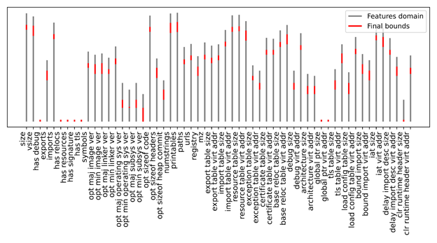
The figure shows an example result that reveals feature intervals (bounds) highly characterizing probable malware configurations.

6.2.2      Minimal Change Analysis

This procedure implements a local search strategy in the feature vector space. The goal is to study the distance between probable malware and benign files by identifying the minimal changes required to features of a benign file to cause the model to classify it as a probable malware (or vice versa). In particular:

1. The procedure starts with a benign instance  (low probability ).
2. The feature bounds are iteratively and minimally extended (bottom-up approach) until an admissible feature vector is found that solves the problem for a new, higher target probability .

This capability highlights weak separators in the ensemble model and potential strategies for attackers to bypass classification. Typically, the first iterations find no models, and the bounds are slowly incremented. If necessary, multiple rounds on all features are performed. Eventually, the optimization that is able to find a solution updates the bounds, so that a sample with probability M is found.

The sample figure shows a depiction of the domain extension process. Gray bars represent domains after the extension. Green dots represent the starting instance features’ values, and red dots represent one admissible solution for target probability.

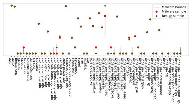
In the provided example, the feature domains are similar for both classifications (malware and benign files), with the exception of a single feature. This distinction allows for the identification of a region within the feature space that influences the model’s classification. From this, we can determine the minimal modification required to alter the model’s behavior and identify the most critical features driving the classification decision.

7       References

• Madden, Samuel. “Lab Data.”, Intel Berkeley Research Lab. 28 Febbraio-5 Aprile 2004. (https://db.csail.mit.edu/labdata/labdata.html).
• https://arxiv.org/abs/2505.10961
• https://arxiv.org/abs/2310.01152

8       Publications

• Gabriele Penzotti, Eleonora Iotti, Alessio Russo, Emanuele Indolfi, Luca Veltri, Francesco Zanichelli, “Challenges in Machine Learning Based Software Vulnerability Assessment”, Challenges of Software Verification Symposium, June 5-6, 2025, Venice, Italy
• Alessio Russo, Eleonora Iotti, Alessandro Dal Palù. Answer Set Programming for Feature-Based Explanation of Malware Prediction. Proceedings of the 40th Italian Conference on Computational Logic (CILC 2025).

8.1      Submitted articles

• Gabriele Penzotti, Eleonora Iotti, Alessio Russo, Emanuele Indolfi, Luca Veltri, Francesco Zanichelli. Challenges in Machine Learning Based Software Vulnerability Assessment. Submitted to “Challenges of Software Verification 2025” Special Issue of “International Journal on Software Tools for Technology Transfer (STTT)”, Springer

---

[1] https://eclipse.dev/paho/

[2] https://github.com/eclipse-paho/paho.mqtt.java

[3] https://mosquitto.org

[4] https://eclipse.dev/paho/

[5] https://github.com/eclipse-paho/paho.mqtt.java

[6] https://eclipse.dev/paho/components/mqtt-sn-transparent-gateway/

[7] https://xgboost.readthedocs.io/en/stable/

[8] https://auto.gluon.ai/stable/index.html

[9] https://db.csail.mit.edu/labdata/labdata.html